Convolutional Neural Networks
NYU K12 STEM Education: Machine Learning (Day 7)

Images in Computer
- Images are stored as arrays of quantized numbers in computers
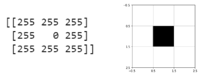
Gray Scale Images
- Gray scale image: 2D matrices with each entry specifying the intensity (brightness) of a pixel
- Pixel values range from 0 to 255, 0 being the darkest, 255 being the brightest
Color Images:
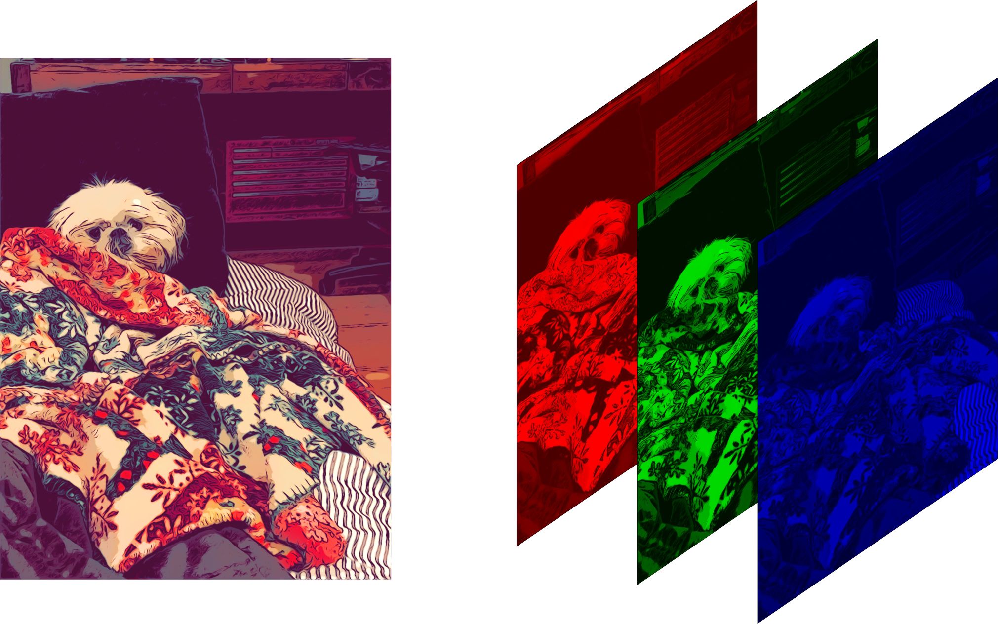
- Color image: 3D array, 2 dimensions for space, 1 dimension for color
- Can be thought of as three 2D matrices stacked together into a cube, each 2D matrix specify the amount of each color: Red,Green, Blue value at each pixel
Limits of Fully Connected Network
- In MNIST, we used a fully connected network, in which each neuron in the hidden layer is connected to all \(28 \times 28 = 784\) pixels
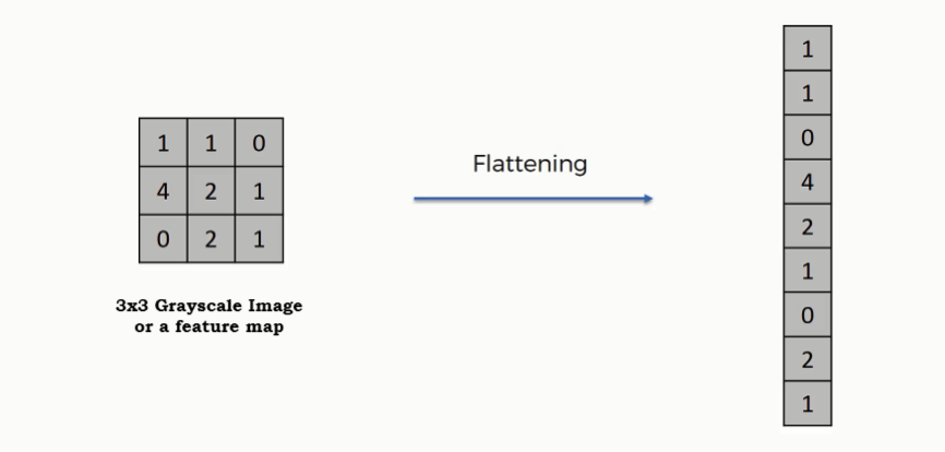
- Higher definition images often contain millions of pixels \(\rightarrow \) It is not practical to use fully connected network
- Fully connected network treat each individual pixel as a feature, it does not utilize the positional relationship between pixels
Convolution
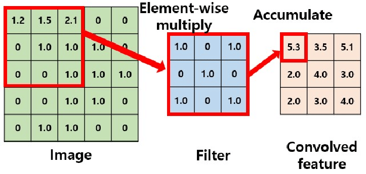
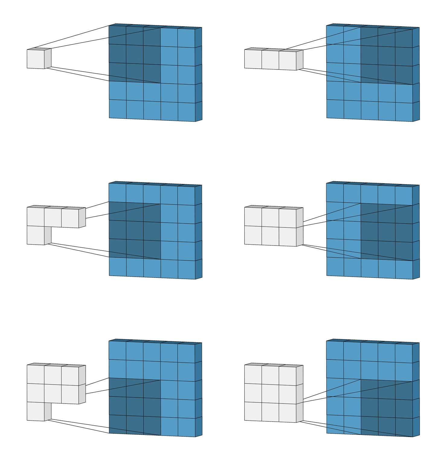
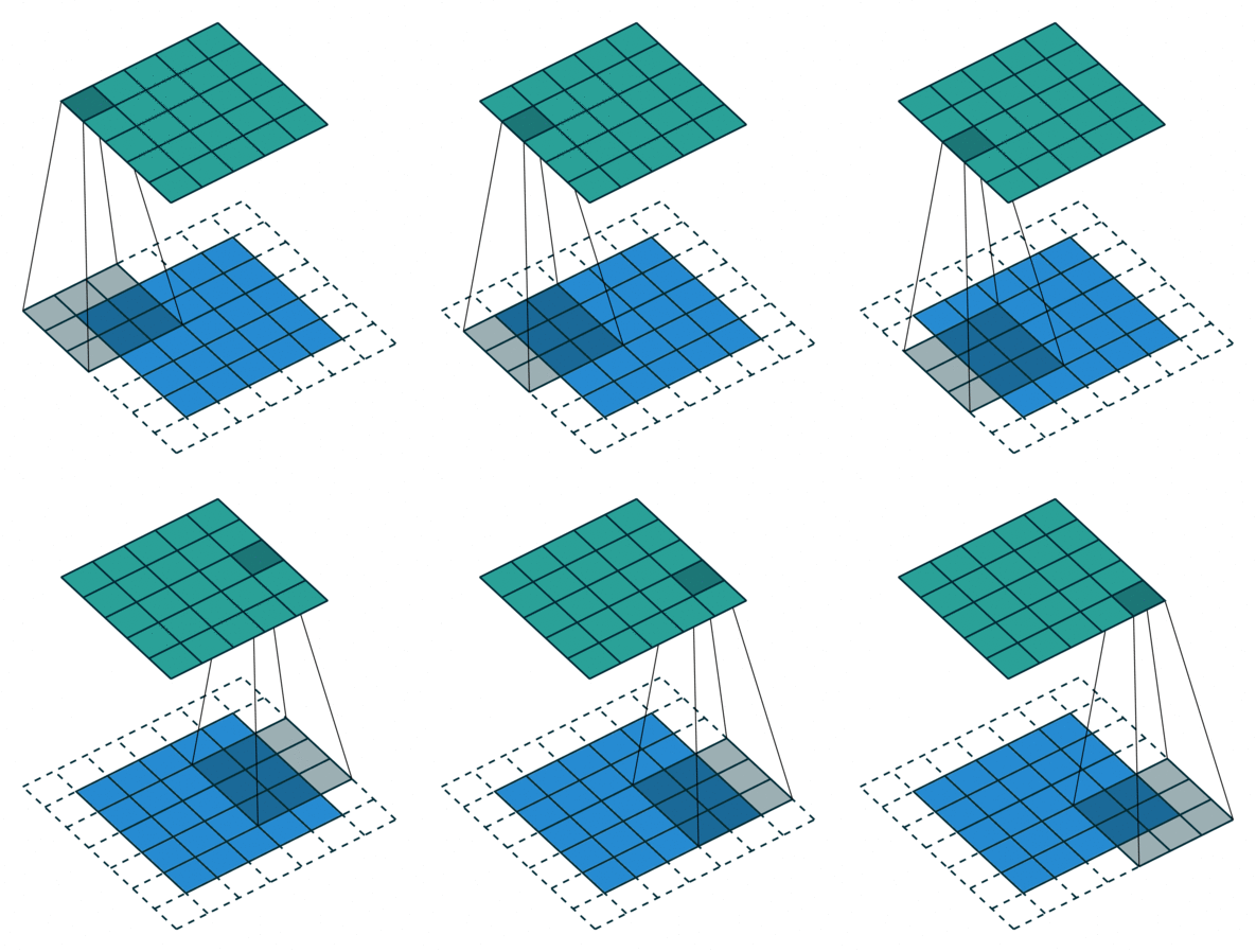
An operation on an image(matrix) X with a kernel W
\[ Z = X \circledast W \]
Why Convolution?
- With convolution, each output pixel depends on only the neighboring pixels in the input
- This allows us to learn the positional relationship between pixels
- Use of different kernels allows us to detect features
Convolution for Multiple Channels
- A kernel for each channel. Could be same kernel, or different
- Perform a convolution for each of the channel, with the respective kernel
- Sum the results

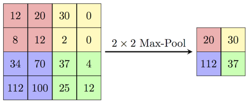
Max-pooling
- Down-samples the inputs
- Provides translation invariance. Why?
- Apply after activation!
Data-augmentation
- Image classification is a difficult task
- We need more data!
- Labeling is expensive and time-consuming.
- How can we create new images?
Examples:
- Mirroring
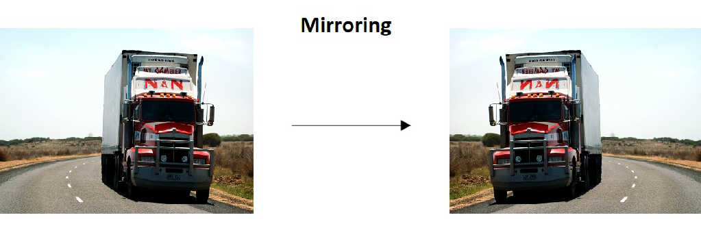
- Rotation and Translation

- Random Cropping
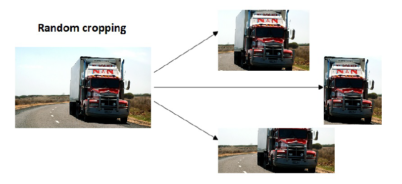
- Color Shifting
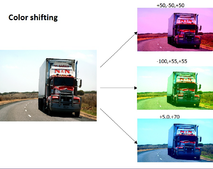
Data Normalization
- Given the dataset \((x_i, y_i) \) for \(i = 1, 2, \cdots, N\)
-
Mean:
\[ \bar{x} = \frac{1}{N} \sum^{N}_{i=1} x_i \]
-
Variance:
\[ \sigma^{2} = \frac{1}{N} \sum^{N}_{i=1} (x_i - \bar{x})^{2} \]
-
Standard deviation:
\[ \sigma = \sqrt{\sigma^2} \]
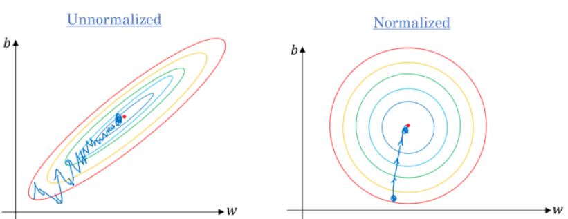
- Normalization : Replace each \(x_i\) by \(x_i’ = \frac{x_i - \bar{x}}{\sigma} \)
- The new dataset will have a mean of \(0\) and a variance of \(1\).
Batch Normalization
- We normalize the inputs to the network. Why not do that for the inputs to the hidden layers?
- Batch norm: normalize the inputs to a layer for each mini-batch.
- Apply before activation!
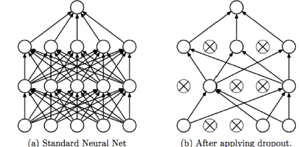
Dropout
- Patented by Google
- Randomly disable neurons and their connections between each other.
- Reduce complex co-adaptive relationships between neurons.
- This is the same as using a neural network with the same amount of layers but less neurons per layer.
- The more neurons the more powerful the neural network is, and the more likely it is to overfit.
- This also means that the model can not rely on any single feature, therefore would need to spread out the weights.
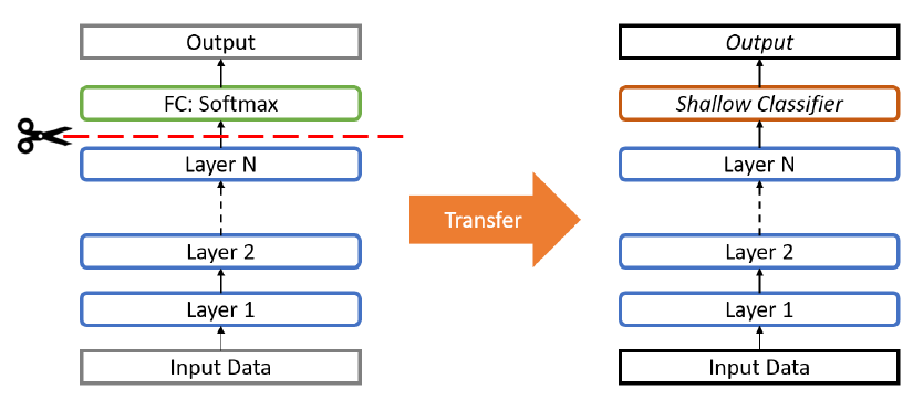
Transfer Learning
- You can freeze the early layers and replace the last few layers to match your own application needs (e.g. different number of classes, different activation functions).
- Only train the replaced layers and use the weights of the early layers ”as-is”.
- This is similar to transferring the knowledge from one network to another, thus the name transfer learning.
