Neural Networks
NYU K12 STEM Education: Machine Learning (Day 6)

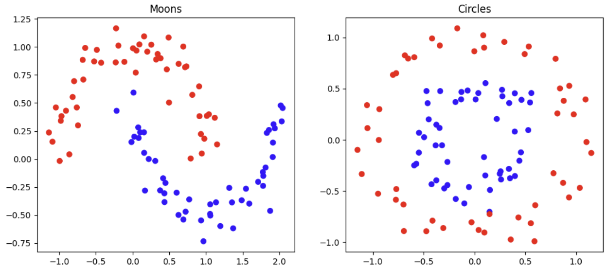
Limitations of Linear Classifiers
- Much more complex dataset are difficult to classify with simple classifiers
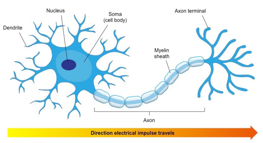
Neuron
Biological Neuron
- A neuron can receive electrochemical signals from other neurons;
- A neuron fires once its accumulated electric charge passes a certain threshold.
- Neurons that fire together wire together.
Mathematical Neuron - Perceptron
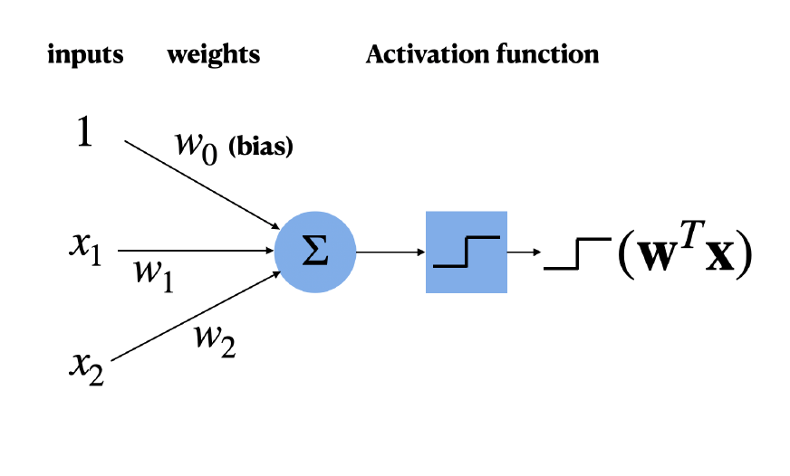
Relation to Logistic Regression
-
What if we use the sigmoid function as the activation?
\[ f(x) = \sigma(w^Tx) \]
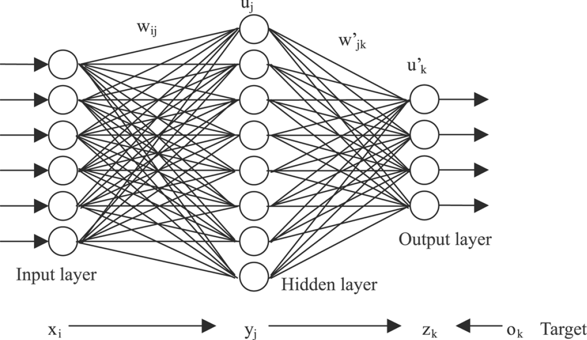
Multi-layer Perceptron (MLP)
- We need more neurons and we need to connect them together!
- Many ways to do that…
- Today: multi-layer perceptron/fully connected feed-forward network.
MLP Example
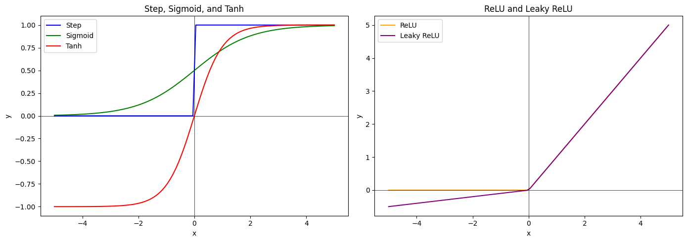
Activation Functions
- Different activation functions have different impact on the behaviour of the neuron.
Deep Neural Network
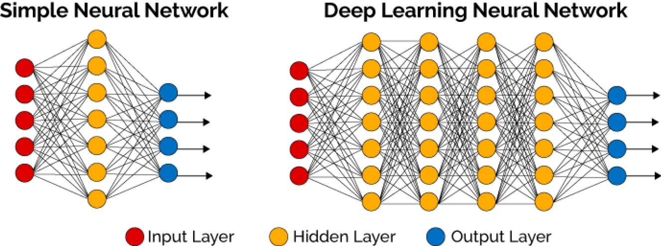
More about MLPs
- Many choices for the activation function: Sigmoid, Tanh, ReLU, Softmax, etc.
- Many choices for the number of hidden layers and the number of neurons per layer.
- MLPs can approximate any continuous function given enough data.
- MLPs can overfit, but we know many effective ways of regularization.
Deep Learning
- What does deep learning mean?
- Deep: Neural network architectures with many hidden layers.
- Learning: Optimizing model parameters given a dataset.
- In general, the deeper the model is, the more parameters we need to learn and the more data is needed.
Large-scale Machine Learning
- For deep learning systems to perform well, large datasets are required
- COCO 330K images
- ImageNet 14 million images
- Challenges:
- Memory limitation: GeForce RTX 2080 Ti has 11 GB memory, while ImageNet is about 300 GB.
- Computation: Calculating gradients for the whole dataset is computationally expensive (slow), and we need to do this many times.
Stochastic Gradient Descent
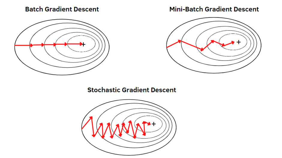
- Idea: Instead of calculating the gradients from the whole dataset, do it only on a subset.
- Randomly select \(B\) samples from the dataset
- The loss for this subset
\[ \hat{J}(w) = \frac{1}{B} \sum^{B}_{i=1} ||y_i - \hat{y_i}||^2 \]
- Update Rule:
\[ \text{Repeat\{} \\ \: w_{\text{new}} = w - \alpha \nabla \hat{J}(w) \\ \text{\}} \]
-
This gives a noisy gradient:
\[ \nabla \hat{J}(w) = \nabla J(w) + \epsilon \]
- SGD: \(B = 1\), gives very noisy gradients
- (batch) GD: \(B = N, \epsilon = 0\), expensive to compute
- Mini-batch GD: Pick a small \(B\), typical values are 32, 64, rarely more than 128 for image inputs
Some Noise Helps
- Even if we can, we rarely set \(B = N\). In fact, some noise in the gradients might help to
- escape from local minima,
- escape from saddle points, and
- improve generalization
Overparameterized Models
- Modern deep learning models are heavily overparameterized, i.e. the number of learnable parameters is much larger than the number of the training samples.
- ResNet: State-of-the-art vision model, 10-60 million parameters
- GPT-3: State-of-the-art language model, 175 billion parameters
- Conventional wisdom: Such models overfit.
- It is not the case in practice!
