Linear Classification
NYU K12 STEM Education: Machine Learning (Day 4)

Classification
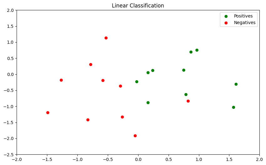
Given the dataset \((x_i , y_i)\) for \(i = 1, 2, \cdots , N\) , find a function \(f (x )\) (model) so that it can predict the label \(\hat{y}\) for some input \(x\), even if it is not in the dataset, i.e. \(\hat{y} = f (x)\)
- Positive : \(y = 1\)
- Negative : \(y = 0\)

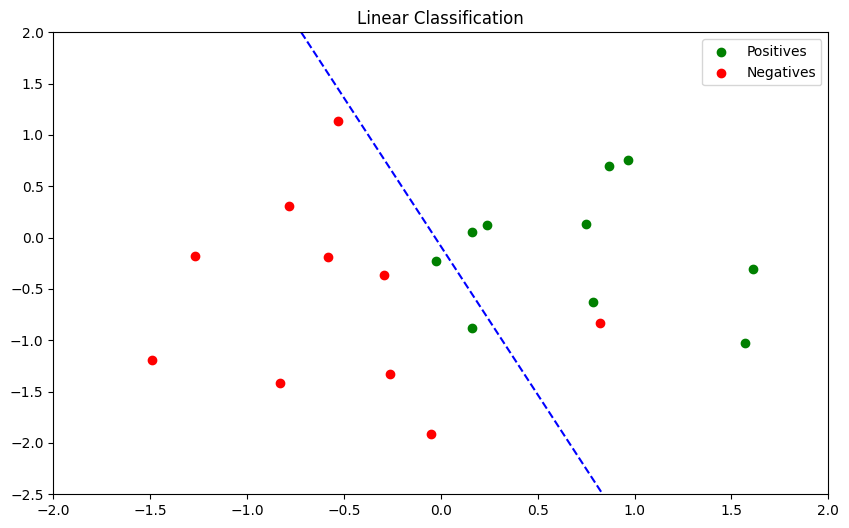
Decision Boundary
-
Evaluation metric :
\[ \text{Accuracy} = \frac{\text{Number of correct prediction}}{\text{Total number of prediction}} \]

Need for a new model
-
What would happen if we used the linear regression model:
\[ \hat{y} = w_0 + w_1x \]
- \(y\) is \(0\) or \(1\)
- \(\hat{y}\) will take any value between \(-\infty\) and \(\infty\)
- It will be hard to find \(w_0\) and \(w_1\) that make the prediction \(\hat{y}\) match the label \(y\)
Sigmoid Function
-
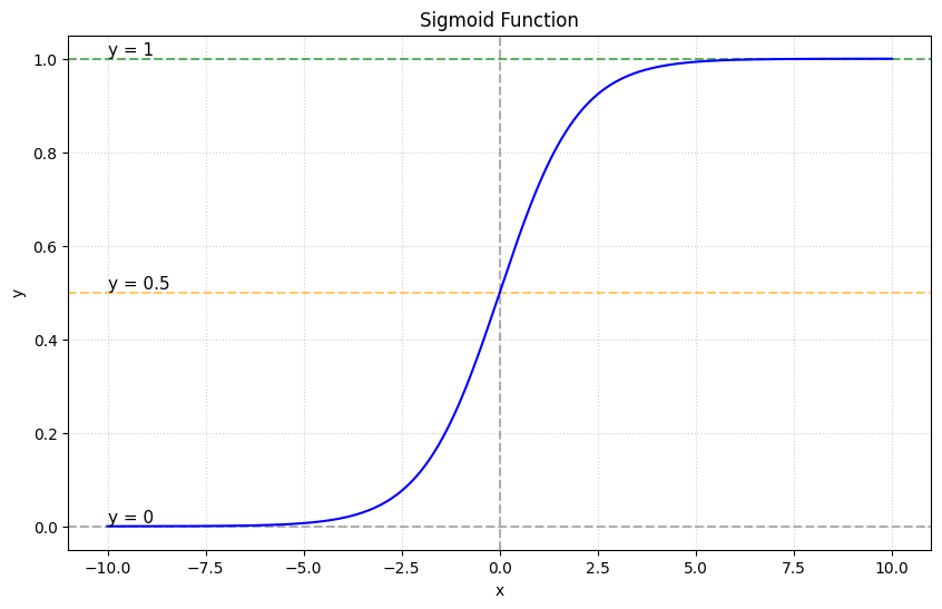
By appling the sigmoid function, we enforce \(0 \le \hat{y} \le 1\)
\[ \hat{y} = \text{sigmoid}(w_0 + w_1x) = \frac{1}{1 + e^{-(w_0 + w_1x)}} \]

Binary Cross Entropy Loss
-
Binary Cross Entropy Loss:
\[ \text{Loss} = \frac{1}{N} \sum^{N}_{i=1} \left[ -y_i \log \hat{y_i} - (1 - y_i) \log (1 - \hat{y_i}) \right] \]
-
If \(y_i = 0\):
\[ \left[ -y_i \log \hat{y_i} - (1 - y_i) \log (1 - \hat{y_i}) \right] = - \log (1 - \hat{y_i}) \]
-
If \(y_i = 1\):
\[ \left[ -y_i \log \hat{y_i} - (1 - y_i) \log (1 - \hat{y_i}) \right] = - \log (\hat{y_i}) \]
MSE vs Binary Cross Entropy Loss
- MSE of a logistic function has many local minima
- The Binary Cross Entropy loss has only one minimum
Classifier
\[ \hat{y} = \text{sigmoid}(w_0 + w_1x) = \frac{1}{1 + e^{-(w_0 + w_1x)}} \]
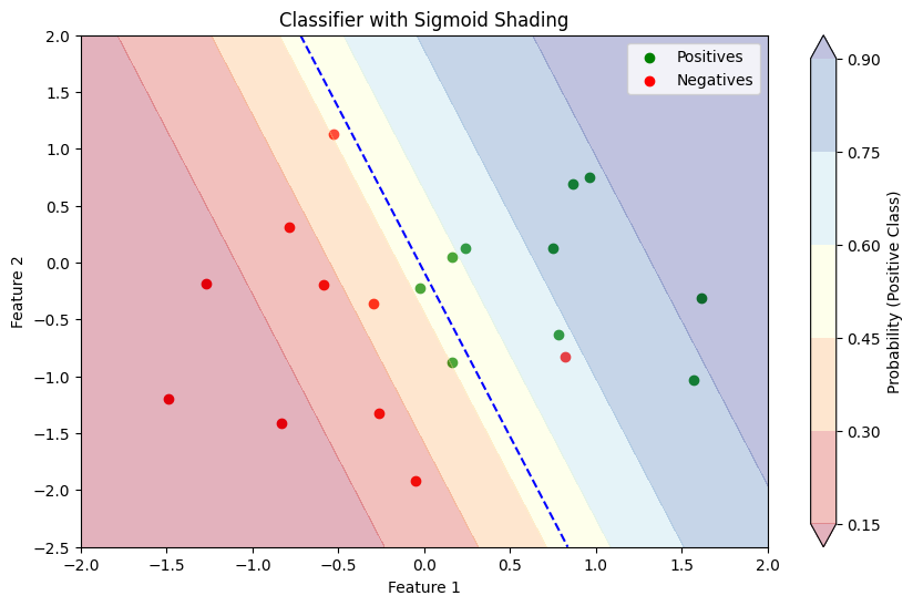
- How to deal with uncertainty?
- Thanks to the sigmoid, \(\hat{y} = f (x)\) is between \(0\) and \(1\)
- If \(\hat{y}\) is close to \(0\), the data is probably negative
- If \(\hat{y}\) is close to \(1\), the data is probably positive
- If \(\hat{y}\) is around \(0.5\), we are not sure.

Decision Boundary
- Once, we have a classifier outputting a score \(0 < \hat{y} < 1\), we need to create a decision rule.
- Let \(0 < t < 1\) be a threshold:
- If \(\hat{y} > t\), \(\hat{y}\) is classified as positive
- If \(\hat{y} < t\), \(\hat{y}\) is classified as negative

Performance metrics for a classifier:
- Accuracy of a classifier: percentage of correct classification
- Why accuracy alone is not a good measure for assessing the model?
- Example: A rare disease occurs 1 in ten thousand people
- A test that classifies everyone as free of the disease can achieve 99.999% accuracy when tested with people drawn randomly from the entire population
Types of Errors in Classification
- Correct predictions:
- True Positive (TP) : Predict \(\hat{y} = 1\) when \(y = 1\)
- True Negative (TN) : Predict \(\hat{y} = 0\) when \(y = 0\)
- Two types of errors:
- False Positive/ False Alarm (FP): \(\hat{y} = 1\) when \(y = 0\)
- False Negative/ Missed Detection (FN): \(\hat{y} = 0\) when \(y = 1\)
Metrics:
-
Sensitivity/Recall/TPR (How many positives are detected among all positive?)
\[ \frac{\text{TP}}{\text{TP} + \text{FN}} \]
-
Precision (How many detected positives are actually positive?)
\[ \frac{\text{TP}}{\text{TP} + \text{FP}} \]
Multiclass Classification
-
Previous Model:
\[ f(x) = \sigma(\phi(x)w) \]
- Representing Multiple Classses:
- One-hot / 1-of-K vectors, ex : 4 Class
- Class 1 : \(y = [1,0,0,0]\)
- Class 2 : \(y = [0,1,0,0]\)
- Class 3 : \(y = [0,0,1,0]\)
- Class 4 : \(y = [0,0,0,1]\)
-
Multiple outputs:
\[ f(x) = \text{softmax}(\phi(x)W) \]
- Shape of \(\phi(x)W\): \((N, K) = (N, D) \times (D, K) \)
-
Softmax:
\[ \text{softmax}(z_k) = \frac{e^{z_k}}{\sum_j e^{z_j}} \]
-
Softmax Example:
\[ z = \begin{bmatrix}-1 \\ 2 \\ 1 \\ -4 \end{bmatrix} \]
\[ \text{softmax}(z) = \begin{bmatrix}\frac{e^{-1}}{e^{-1} + e^{2} + e^{1} + e^{-4}} \\ \frac{e^{2}}{e^{-1} + e^{2} + e^{1} + e^{-4}} \\ \frac{e^{1}}{e^{-1} + e^{2} + e^{1} + e^{-4}} \\ \frac{e^{-4}}{e^{-1} + e^{2} + e^{1} + e^{-4}} \end{bmatrix} \approx \begin{bmatrix}0.035 \\ 0.704 \\ 0.259 \\ 0.002 \end{bmatrix} \]
Cross-entropy
- Multple Outputs: \( \hat{y_i} = \text{softmax}(\phi(x_i)W)\)
-
Cross-Entropy:
\[ J(W) = - \sum^{N}_{i=1} \sum^{K}_{k=1} y_{ik} \log (\hat{y_{ik}}) \]
-
Example, \(K = 4\), if \(y_i = [0, 0, 1, 0]\) then,
\[ \sum^{K}_{k=1} y_{ik} \log (\hat{y_{ik}}) = \log (\hat{y_{i3}}) \]
