Overfitting and Regularization
NYU K12 STEM Education: Machine Learning (Day 3)

Polynomial Fitting
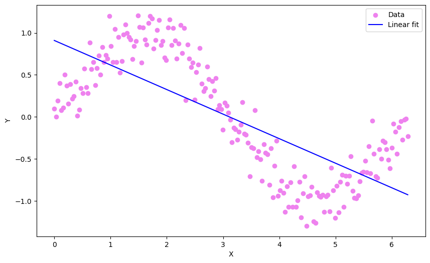
- We have been using straight lines to fit our data. But it doesn’t work well every time
- Some data have more complex relation that cannot be fitted well using a straight line
-
Polynomial: A sum of different powers of a variable
Examples: \(y = x^2 + 2, y = 5x^3 − 3x^2 + 4\)

- Polynomials of \(x\): \(\hat{y} = w_0 + w_1x +w_2x^2 + w_3x^3 + \cdots + w_Mx^M\)
- \(M\) is called the order of the polynomial.
- The process of fitting a polynomial is similar to linearly fitting multivariate data.
- Rewrite in matrix-vector form \[ \begin{bmatrix} \hat{y_1} \\ \hat{y_2} \\ \vdots \\ \hat{y_N} \end{bmatrix} = \begin{bmatrix}1 & x_{1} & x_{1}^2 & \cdots & x_{1}^M \\ 1 & x_{2} & x_{2}^2 & \cdots & x_{2}^M \\ \vdots & \vdots & \vdots & \ddots & \vdots \\ 1 & x_{N} & x_{N}^2 & \cdots & x_{N}^M\end{bmatrix} \begin{bmatrix}w_0 \\ w_1 \\ \vdots \\ w_M \end{bmatrix} \]
- This can still be written as: \(\hat{Y} = Xw\)
- Loss: \[ J(w) = \frac{1}{N} ||Y - Xw ||^2 \]
- The \(i^{th}\) row of the design matrix \(X\) is simply a transformed feature: \[ \phi(x_i) = (1, x_i, x_i^2, \cdots, x_i^M) \]
- Original Design Matrix: \[ \begin{bmatrix} 1 & x_1 \\ 1 & x_2 \\ \vdots & \vdots \\ 1 & x_N \end{bmatrix} \]
- Design matrix after feature transformation: \[ \begin{bmatrix}1 & x_{1} & x_{1}^2 & \cdots & x_{1}^M \\ 1 & x_{2} & x_{2}^2 & \cdots & x_{2}^M \\ \vdots & \vdots & \vdots & \ddots & \vdots \\ 1 & x_{N} & x_{N}^2 & \cdots & x_{N}^M\end{bmatrix} \]
- For the polynomial fitting, we just added columns of features that are powers of the original feature.
Overfitting
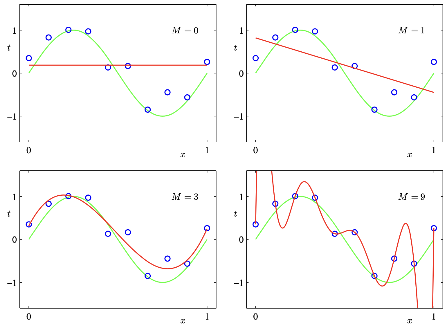
- We learned how to fit our data using polynomials of different order
- With a higher model order, we can fit the data with increasing accuracy
- As you increase the model order, at certain point it is possible find a model that fits your data perfectly (ie. zero error)
- What could be the problem?
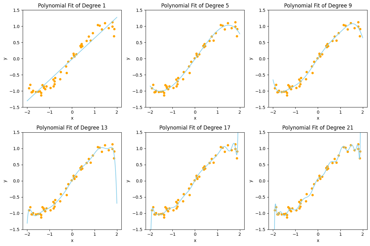
- Which of these model do you think is the best? Why?
- The problem is that we are only fitting our model using data that is given
- Data usually contains noise
- When a model becomes too complex, it will start to fit the noise in the data
- What happens if we apply our model to predict some data that the model has never seen before? It will not work well.
- This is called over-fitting.
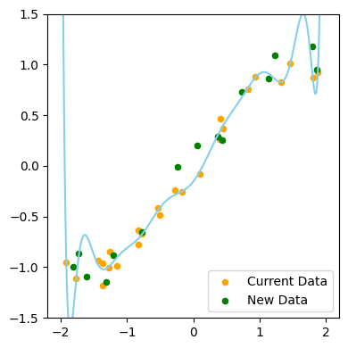
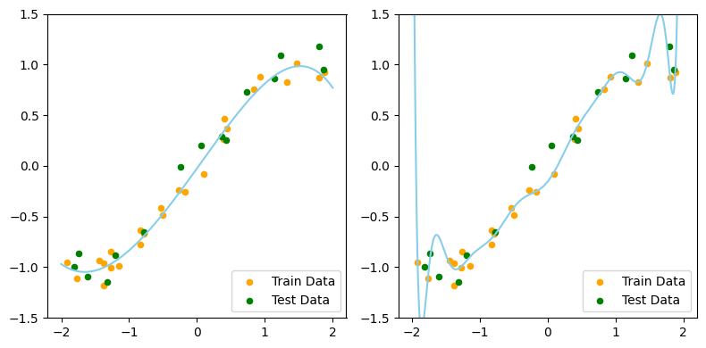
- Split the data set into a train set and a test set
- Train set will be used to train the model
- The test set will not be seen by the model during the training process
- Use test set to evaluate the model when a model is trained
- With the training and test sets shown, which one do you think is the better model now?
Train and Test Error
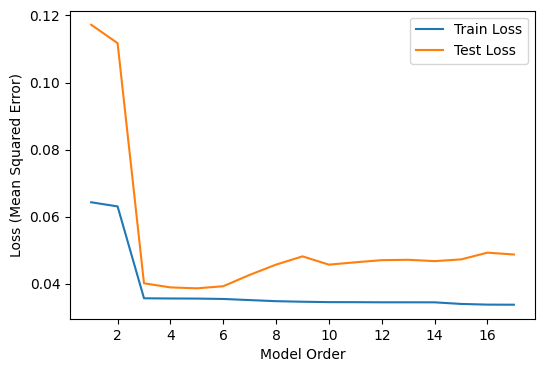
- Plot of train error and test error for different model order
- Initially both train and test error go down as model order increase
- But at a certain point, test error start to increase because of overfitting
Regularization
- Regularization: methods to prevent overfitting
- Is there another way?
- Solution: We can change our cost function.
Weight Based Regularization
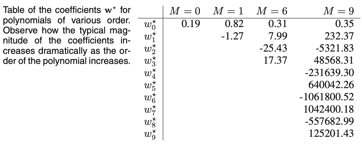
- Looking back at the polynomial overfitting
- Notice that weight-size increases with overfitting
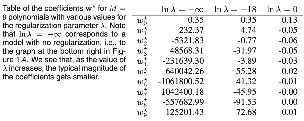
New Cost Function: \[ J(w) = \frac{1}{N} ||Y - Xw ||^2 + \lambda ||w||^2 \]
- Penalize complexity by simultaneously minimizing weight values.
- We call \(\lambda\) a hyper-parameter
- \(\lambda\) determines relative importance
Tuning Hyper-parameters
- Motivation: never determine a hyper-parameter based on training data
- Hyper-Parameter: a parameter of the algorithm that is not a model-parameter solved for in optimization. Example: \(\lambda\) weight regularization value vs. model weights (\(w\))
- Solution: split dataset into three
- Training set: to compute the model-parameters (\(w\))
- Validation set: to tune hyper-parameters (\(\lambda\))
- Test set: to compute the performance of the algorithm (MSE)
Non-linear Optimization
- Cannot rely on closed form solutions
- Computation efficiency: operations like inverting a matrix is not efficient
- For more complex problems such as neural networks, a closed-form solution is not always available
- Need an optimization technique to find an optimal solution
- Machine learning practitioners use gradient-based methods
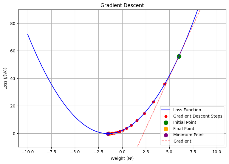
Gradient Descent Algorithm
-
Update Rule:
\[ \text{Repeat\{} \\ w_{\text{new}} = w - \alpha \nabla J(w) \\ \text{\}} \]
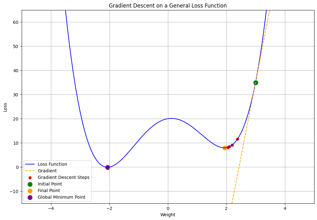
General Loss Function Contours
- Most loss function contours are not perfectly parabolic
- Our goal is to find a solution that is very close to global minimum by the right choice of hyper-parameters
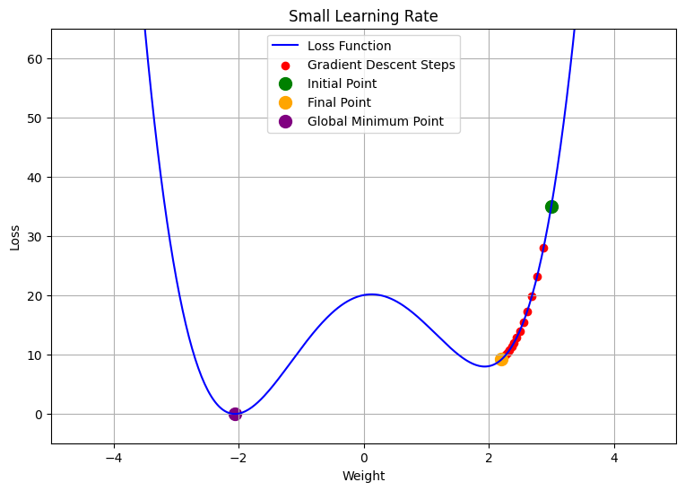
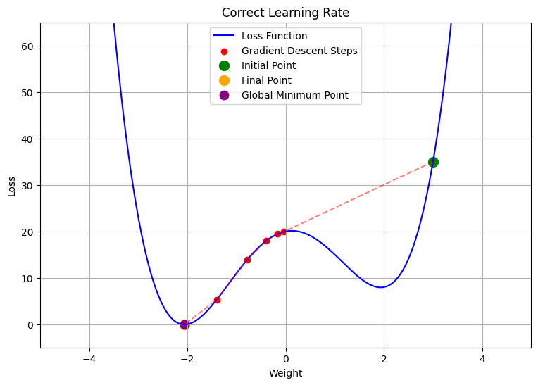
Understanding Learning Rate
- Small Learning Rate:
- Correct Learning Rate:
- Large Learning Rate:
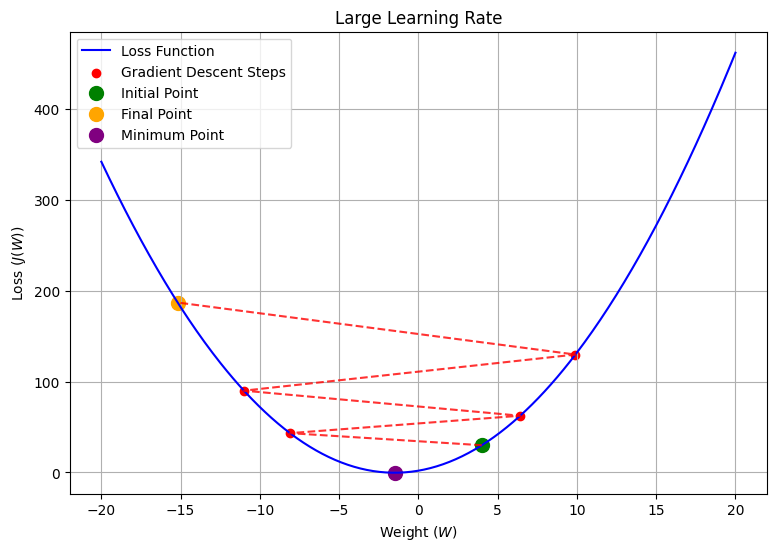
Some Learning Rate Animations:
- Small Learning Rate:
- Correct Learning Rate:
- Large Learning Rate:
