Linear Regression
NYU K12 STEM Education: Machine Learning (Day 2)

Statistics Review
In machine learning, a solid understanding of basic statistical concepts is essential for analyzing data and interpreting model results.
Mean
The mean, or average, is the sum of all the values in a dataset divided by the number of values. It provides a measure of the central tendency of the data.
Formula: \[ \text{Mean} (\mu) = \frac{1}{N} \sum_{i=1}^{N} x_i \]
Example:
For the dataset [2, 4, 6, 8, 10]: \[ \mu = \frac{2 + 4 + 6 + 8 + 10}{5} = 6 \]
Variance
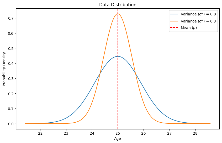
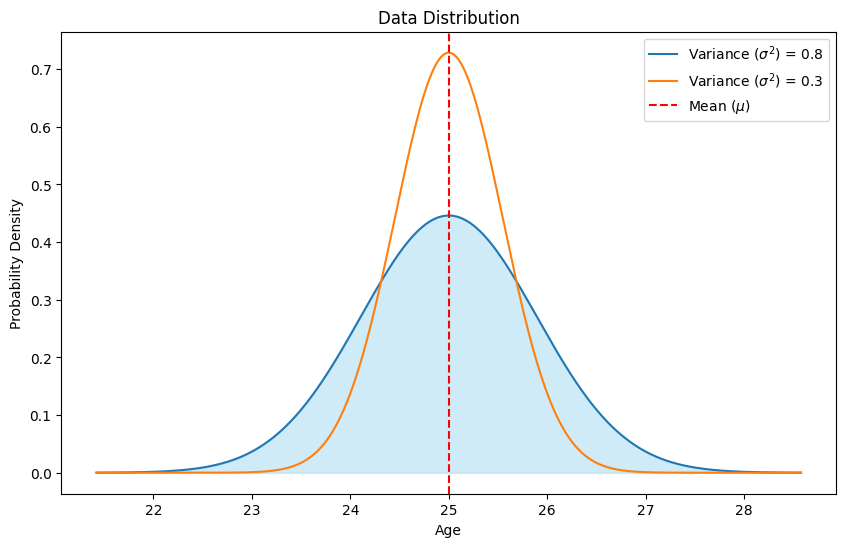
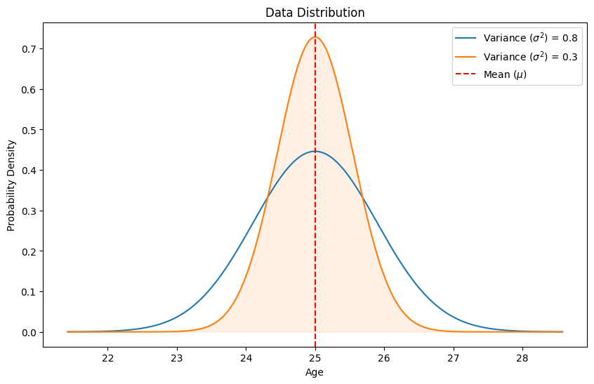
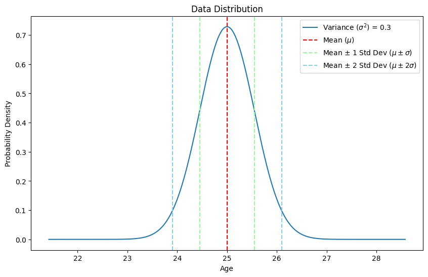
Variance measures the spread of the data points around the mean. It indicates how much the data varies from the mean.
Formula: \[ \text{Variance} (\sigma^2) = \frac{1}{N} \sum_{i=1}^{N} (x_i - \mu)^2 \]
Example:
For the dataset [2, 4, 6, 8, 10]: \[ \sigma^2 = \frac{(2-6)^2 + (4-6)^2 + (6-6)^2 + (8-6)^2 + (10-6)^2}{5} = 8 \]
Mean and Variance Visualization
Standard Deviation
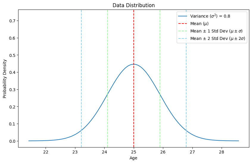
Standard deviation is the square root of the variance. It provides a measure of the spread of the data points in the same units as the data itself.
Formula: \[ \text{Standard Deviation} (\sigma) = \sqrt{\text{Variance}} \]
Example:
Using the variance calculated above: \[ \sigma = \sqrt{8} \approx 2.83 \]
Standard Deviation Visualization
Covariance
Covariance measures the degree to which two variables change together. If the covariance is positive, the variables tend to increase together; if negative, one variable tends to increase when the other decreases.
Formula: \[ \text{Covariance} (\text{Cov}(X, Y)) = \frac{1}{N} \sum_{i=1}^{N} (x_i - \mu_X)(y_i - \mu_Y) \]
Example: For the datasets X = [2, 4, 6] and Y = [3, 6, 9]: \[ \text{Cov}(X, Y) = \frac{(2-4)(3-6) + (4-4)(6-6) + (6-4)(9-6)}{3} = 6 \]

Linear Regression
In a Nutshell…
- Consider a function \(y = 2x + 1 \)
- Here we introduce a new notation \(f (x) = 2x + 1 \)
- What this means is that we have a function \(f (x ) \) which has \(x\) as its variable.
- If we have different \(x\) values we will have different values of \(f(x)\).
Example:
- For \(f (x) = 2x + 1 \) and setting \(x = 1\) we have \(f (x) = 3\)
- For \(f (x) = 2x + 1 \) and setting \(x = 0\) we have \(f (x) = 1\)
- For \(f (x) = 2x + 1 \) and setting \(x = −1.5\) we have \(f (x) = −2\)
- We believe that dataset are representation of underlying models which can be represented as functions of features.
- For example, we can build a model to forecast weather, we can use the features humidity, current temperature and wind speed to estimate what the temperature will be tomorrow.
- Here we have \(f (x)\) representing the tomorrow’s temperature and \(x\) being a vector containing humidity, current temperature and wind speed.
- But many times we do have \(f (x)\) available, our task here is to figure out what \(f (x)\) is using the data available to us.
- Here \(f (x)\) is called a model.
- In other words, we want to find a model that fits the data.
- It would be easier to have a ”framework” of the model ready and find the model parameters using the data.
- \(f (x) = w_1x + w_0\)
- \(f (x) = w_2x^2 + w_1x + w_0\)
- \(f (x) = \frac{1}{e^{−(w_1x+w_0)} + 1}\)
- The numbers \(w_0\), \(w_1\) and \(w_2\) are called model parameters.
- We often write the model as \(f (x ; w)\), stacking all parameters to a vector \(w\).
Structure of a dataset
- In a dataset we have many data.
- We can represent each piece of data as \((x_i,y_i)\), \(i = 1,2,3,\cdots\)
- \(x_i\) is called the feature and \(y_i\) is called the label.
- The relationship between \(x_i\) and \(y_i\) and the model \(f\) is \(f (x_i ) = y_i\)
- For example, if the weather forecast says it will be 21\(^{\circ}\)C (69.8\(^{\circ}\)F) if it turns out to be 22\(^{\circ}\)C (71.6\(^{\circ}\)F) you won’t be yelling at the TV.
How would you fit a line?
Can you find a line that passes through (0, 0) and (1, 1)?
- The ”framework” of the model is \(f (x) = w_1x + w_0\)
- The data is (\(x = 0\), \(f (x ) = y = 0\)) and (\(x = 1\), \(f (x ) = y = 1\)).
- The process of finding a model to fit the data is to find the values of \(w_1\) and \(w_0\).
How would you fit a quadratic curve?
Can you find a quadratic curve that passes through (0, 0), (1, 1) and (−1, 1)?
- The ”framework” of the model is \(f (x) = w_2x^2 + w_1x + w_0\)
- The data is \((x = 0, f (x ) = y = 0)\), \((x = 1, f (x ) = y = 1)\) and \((x =−1,f(x)=y =1)\)
- The process of finding a model to fit the data is to find the values of \(w_2\), \(w_1\) and \(w_0\).
Is Your Model a Good Fit?
- How would you determine if your model is a good fit or not?
- How will you determine this?
- Is there a quantitative way?
- We now introduce a new notation \(f(x_i) = \hat{y_i}\) here the \(\hat{\cdot}\) represents \(f(x_i)\) is a prediction of \(y_i\).
Error Functions
- An error function quantifies the discrepancy between your model and the data.
- They are non-negative, and go to zero as the model gets better.
- Common Error Functions:
- Mean Squared Error: \[ \text{MSE} = \frac{1}{N}\sum^{N}_{i=1}||y_i - \hat{y_i}||^2 \]
- Mean Absolute Error: \[ \text{MAE} = \frac{1}{N}\sum^{N}_{i=1}|y_i - \hat{y_i}| \]
- In later units, we will refer to these as cost functions or loss functions.
Linear Regression
- Linear models: For scalar-valued feature \(x\), this is \(f (x) = w_1x + w_0\)
- One of the simplest machine learning model, yet very powerful.
Least Square Solution
- Model: \(f (x) = w_1x + w_0\)
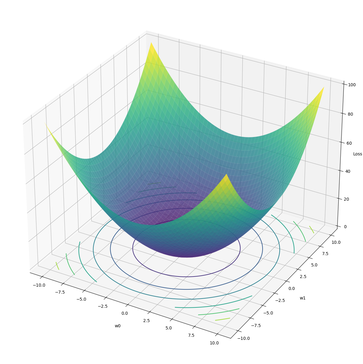
- Loss: \[ J(w_0, w_1) = \frac{1}{N}\sum^{N}_{i=1}||y_i - f(x_i)||^2 \]
- Optimization: Find \(w_0\), \(w_1\) such that \(J(w_0, w_1)\) is the least possible value (hence the name “least square”).
Using Pseudo-Inverse
- For \(N\) data points (\(x_i, y_i\)) we have, \[ \begin{split} \hat{y_1} &= w_0 + w_1x_1 \\ \hat{y_2} &= w_0 + w_1x_2 \\ &\vdots \\ \hat{y_N} &= w_0 + w_1x_N \end{split} \]
- In matrix form we have, \[ \begin{bmatrix}\hat{y_1} \\ \hat{y_2} \\ \vdots \\ \hat{y_N} \end{bmatrix} = \begin{bmatrix} 1 & x_1 \\ 1 & x_2 \\ \vdots & \vdots \\ 1 & x_N \end{bmatrix} \begin{bmatrix}w_0 \\ w_1 \end{bmatrix} \]
- We can write it as \(\hat{Y} = X \times w \). We call \(X\) the design matrix.
- We can put the desired labels in matrix form as well: \[ Y = \begin{bmatrix}y_1 \\ y_2 \\ \vdots \\ y_N \end{bmatrix} \]
- Our goal is to minimize the error between \(Y\) and \(\hat{Y}\) which can be written as \(||Y - \hat{Y}||^2\)
Multilinear Regression
- What if we have multivariate data with \(x\) being a vector?
-
Example: \[ x_i = \begin{bmatrix}x_{i1} \\ x_{i2} \end{bmatrix} \]
\[ \begin{split} \hat{y_1} &= w_0 + w_1x_{11} + w_2x_{12} \\ \hat{y_2} &= w_0 + w_1x_{21} + w_2x_{22} \\ &\vdots \\ \hat{y_N} &= w_0 + w_1x_{N1} + w_2x_{N2} \end{split} \]
- The model can be written as: \( \hat{y_i} = \begin{bmatrix}1 & x_{i1} & x_{i2}\end{bmatrix} \begin{bmatrix}w_0 \\ w_1 \\ w_2 \end{bmatrix} \)
- In matrix-vector form: \( \begin{bmatrix} \hat{y_1} \\ \hat{y_2} \\ \vdots \\ \hat{y_N} \end{bmatrix} = \begin{bmatrix}1 & x_{11} & x_{12} \\ 1 & x_{21} & x_{22} \\ \vdots & \vdots & \vdots \\ 1 & x_{N1} & x_{N2}\end{bmatrix} \begin{bmatrix}w_0 \\ w_1 \\ w_2 \end{bmatrix} \)
- Solution remains the same \(w = (X^T X)^{-1} X^T Y\)
Demos
- Vectorized Programming
- Plotting Functions
- Ice-breaker Dataset
- Linear Regression
- Multivariable Linear Regression
