Introduction to Machine Learning
NYU K12 STEM Education: Machine Learning (Day 1)

Why do we learn Machine Learning?
- Everyone has pretty much heard about, or used Machine Learning (ML) or Artificial Intelligence (AI) like ChatGPT, Siri, Amazon Alexa, etc. It is also mentioned everywhere in the news, and in everyday conversations.
- It is the most recent exciting technology. People say that “AI is the new electricity”. Back then, electricity transformed countless industries like transportation, manufacturing, healthcare, communications and more. Now, AI will bring about an equally big transformation.
- ML Applications can range from (relatively) simple tasks like weather prediction to more complex tasks like self-driving cars.
- Due to this, the demand for Machine Learning skills is very vast.
What is Machine Learning?
Traditional Programming
- Rule-based
- Doesn’t work with complex problems like detecting handwritten digits.

Machine Learning
Machine learning is a field of study that gives computers the ability to learn without being explicitly programmed.


Types of Machine Learning
Supervised Learning
Supervised learning is a type of machine learning where the model is trained on a labeled dataset. This means that for every training example, the model has access to the input data as well as the corresponding output (label). The goal of supervised learning is to learn a mapping from inputs to outputs so that the model can predict the output for new, unseen data.
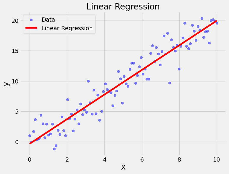
Regression
- Used when the output variable is continuous.
- Linear Regression: Predicts a continuous target variable as a linear combination of input features.
Example: Predicting house prices based on features like size, location, and number of bedrooms.
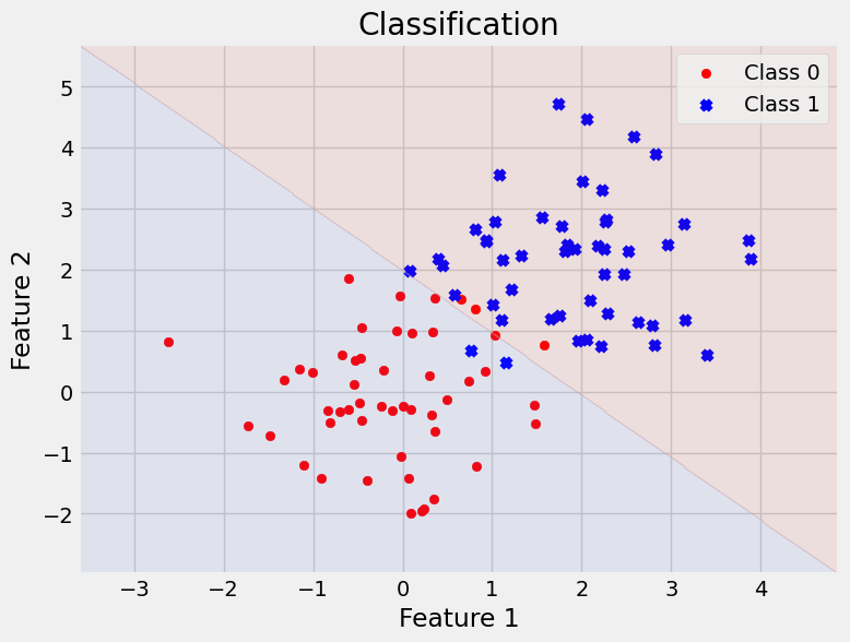
Classification
- Used when the output variable is categorical.
- Logistic Regression: Predicts the probability of a categorical target variable.
Example: Classifying emails as spam or not spam.
Unsupervised Learning
Unsupervised learning is a type of machine learning where the model is trained on data without labeled responses. The goal is to uncover hidden patterns, structures, or relationships in the data. Unlike supervised learning, there are no explicit instructions on what the output should look like, and the algorithm must infer the patterns and structure from the input data.
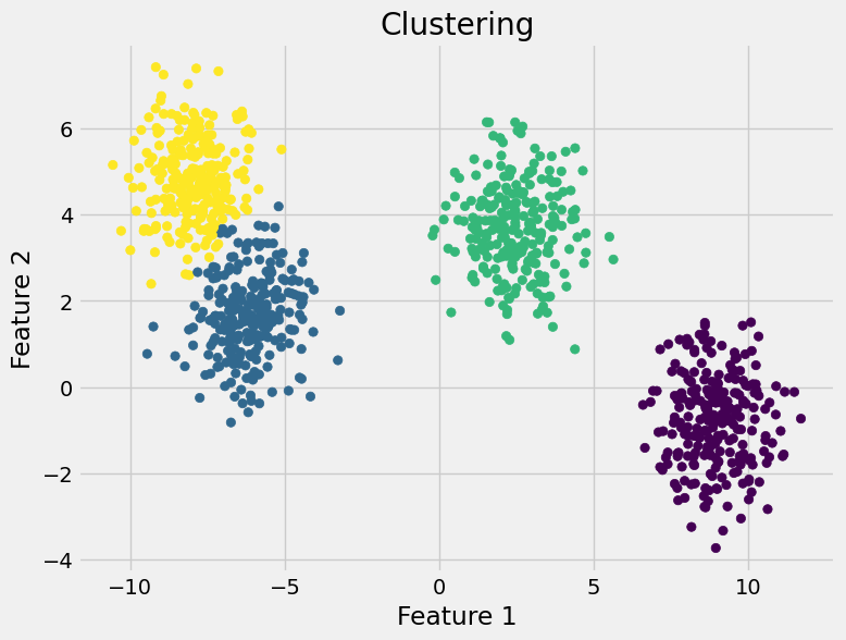
Clustering
- Group similar data points into clusters.
Example: Retailers use clustering to create personalized marketing campaigns.
Reinforcement Learning
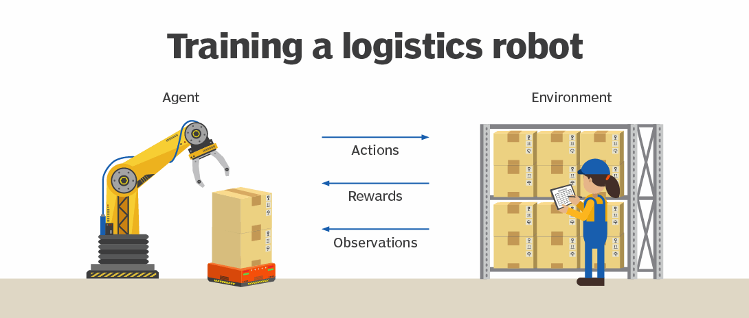
Reinforcement Learning (RL) is a type of machine learning where an agent learns to make decisions by performing actions in an environment to maximize cumulative reward. Unlike supervised learning, where the model is trained with labeled data, reinforcement learning relies on a trial-and-error approach, where the agent interacts with the environment and receives feedback in the form of rewards or penalties.
Examples:
- Training agents to play and excel in video games or board games (e.g., AlphaGo, Dota 2).
- Controlling robotic systems to perform tasks like walking, grasping objects, or navigating.
- Developing self-driving cars that can navigate roads, avoid obstacles, and make decisions in real-time.
Examples
Digit Recognizer
A digit recognizer is a machine learning model designed to classify handwritten digits (0-9) based on their pixel values. One of the most well-known and widely used datasets for this task is the MNIST dataset. The MNIST dataset was created by Yann LeCun, a professor at New York University (NYU), and a prominent figure in deep learning and a pioneer of convolutional neural networks (CNNs).
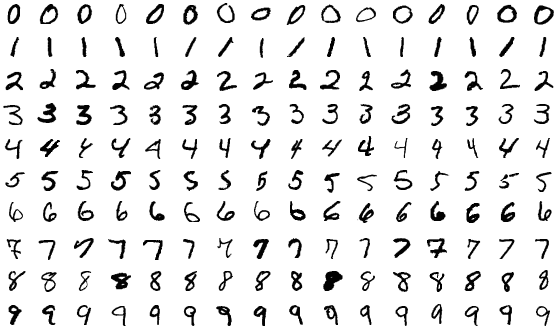
Machine learning models, particularly deep learning models like Convolutional Neural Networks (CNNs), excel at recognizing handwritten digits because they learn patterns directly from large datasets. By automatically extracting features such as edges, textures, and shapes from raw pixel data, these models adapt to various handwriting styles and handle noise and distortions. Their ability to capture complex non-linear relationships in the data makes them robust to variations in size, angle, and thickness of digits. In contrast, expert systems rely on predefined rules and if-else conditionals, which are inflexible and impractical for the vast range of handwriting variations (for instance, rules might include “if the center column has a certain number of black pixels, it might be a ‘1’”). These systems perform well only on scenarios explicitly programmed, struggle with generalization, and become unmanageably complex with numerous conditions. Consequently, machine learning approaches offer superior performance and scalability in handwritten digit recognition compared to rule-based expert systems.
CIFAR-10
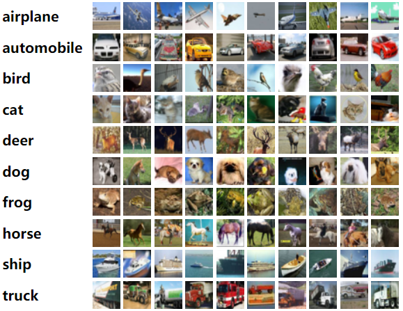
For complex image recognition tasks like those in the CIFAR-10 dataset, machine learning approaches, particularly Convolutional Neural Networks, are indispensable. They offer powerful automatic feature extraction, scalability, and generalization capabilities that manual rule-based systems cannot match. This makes machine learning the only viable approach for handling the complexity and variability inherent in such image datasets.
These Cats Do Not Exist
ML models can also be used to generate images. For instance, these images of cats are not of real cats; they were created by an ML model called Generative Adversarial Network (GAN).

DALL.E
Models like DALL.E can generate new images based on textual prompts. This model extends the capabilities of existing language-based AI systems by generating highly realistic and diverse images across a wide range of concepts, from everyday objects to abstract concepts. DALL·E achieves this by learning a multimodal representation of images and text, allowing it to understand and synthesize complex visual concepts described in natural language.


ChatGPT
And we all know and have used the ChatGPT model. ChatGPT is an advanced conversational AI model based on the GPT (Generative Pre-trained Transformer) architecture. It is designed to engage in natural and contextually relevant conversations with users.
Precalculus Review
Why do we learn Vectors and Matrices?
Studying vectors and matrices is crucial in machine learning because they form the basis for data representation, model implementation, and optimization. Many machine learning algorithms, such as linear regression and neural networks, rely heavily on linear algebra operations like matrix multiplication and dot products. Understanding vectors and matrices helps in representing datasets, performing essential calculations, optimizing model parameters, and interpreting model behavior, making them indispensable for both theoretical understanding and practical application in machine learning.

Matrices
A matrix is a rectangular array of numbers (or other mathematical objects). For example:
\( A = \begin{bmatrix} 1 & 3 \\ 2 & -1 \end{bmatrix} \)
Size of a Matrix
The size of a matrix is defined by the number of rows and columns it contains. The above matrix \(A \) has 2 rows and 2 columns, so the size of the matrix is \( 2 \times 2 \)
Example:
\( M = \begin{bmatrix} 1 & 3 \\ 2 & -1 \\ -4 & 5 \end{bmatrix} \)
\( \therefore M \) is a matrix of size \( 3 \times 2 \)
In general, a matrix \(A \) of size \( m \times n\) is given as,
\( \begin{bmatrix} a_{11} & a_{12} & \cdots & a_{1n} \\ a_{21} & a_{22} & \cdots & a_{2n} \\ \vdots & \vdots & \ddots & \vdots \\ a_{m1} & a_{m2} & \cdots & a_{mn} \end{bmatrix} \),
where \(a_{ij} \) represents the \( i^{th} \) row and \( j^{th} \) column element.
For example, the element \( m_{31} \) in the above matrix \( M \) is equal to \( -4 \).
Matrix Addition and Subtraction
Matrices of the same size may be added together, element-wise. For example:
\( A = \begin{bmatrix} 1 & 1 \\ 2 & 1 \end{bmatrix} \), \( B = \begin{bmatrix} 0 & 8 \\ 7 & 1 \end{bmatrix} \)
\( \therefore C = A + B = \begin{bmatrix} 1+0 & 1+8 \\ 2+7 & 1+1 \end{bmatrix} = \begin{bmatrix} 1 & 9 \\ 9 & 2 \end{bmatrix} \)
Similarly, matrices of the same size may be subtracted together, element-wise. For example:
\( A = \begin{bmatrix} 1 & 1 \\ 2 & 1 \end{bmatrix} \), \( B = \begin{bmatrix} 0 & 8 \\ 7 & 1 \end{bmatrix} \)
\( \therefore D = A - B = \begin{bmatrix} 1-0 & 1-8 \\ 2-7 & 1-1 \end{bmatrix} = \begin{bmatrix} 1 & -7 \\ -5 & 0 \end{bmatrix} \)
Matrix Scalar Multiplication
Matrices can be scaled by a number. The resulting matrix is computed element-wise. This operation is called scalar multiplication. For example:
\( A = \begin{bmatrix} 1 & 1 \\ 2 & 1 \end{bmatrix} \), \( c = 3 \)
\( \therefore c \cdot A = \begin{bmatrix} 1 \times 3 & 1 \times 3 \\ 2 \times 3 & 1 \times 3 \end{bmatrix} = \begin{bmatrix} 3 & 3 \\ 6 & 3 \end{bmatrix} \)
Transpose of a Matrix
The transpose of a matrix is formed by swapping rows and columns. For example:
\( M = \begin{bmatrix} 1 & 3 \\ 2 & -1 \\ -4 & 5 \end{bmatrix} \)
\( M^T = \begin{bmatrix} 1 & 2 & -4 \\ 3 & -1 & 5 \end{bmatrix} \)
A transposed matrix is denoted as \( M^T \).
Vectors
Matrices with a single row are called row vectors. A row vector is a \( 1 \times n\) matrix, consisting of a single row of \( n \) elements. For example:
\( U = \begin{bmatrix} 1 & 2 & 3\end{bmatrix} \)
Matrices with a single column are called column vectors. A column vector is a \( n \times 1 \) matrix, consisting of a single column of \( n \) elements. (We consider column vectors by default)
For example:
\( V = \begin{bmatrix} 1 \\ 2 \\ 3\end{bmatrix} \)
Vector Addition and Subtraction
Vectors of the same dimensions may be added together, element-wise. For example:
\( V = \begin{bmatrix} 1 \\ 2 \\ 3\end{bmatrix} \), \( W = \begin{bmatrix} 4 \\ 5 \\ 6\end{bmatrix} \)
\( \therefore X = V + W = \begin{bmatrix} 1 + 4 \\ 2 + 5 \\ 3 + 6\end{bmatrix} = \begin{bmatrix} 5 \\ 7 \\ 9\end{bmatrix} \)
Similarly, vectors of the same dimensions may be subtracted together, element-wise. For example:
\( \therefore Y = W - V = \begin{bmatrix} 4 - 1 \\ 5 - 2 \\ 6 - 3\end{bmatrix} = \begin{bmatrix} 3 \\ 3 \\ 3\end{bmatrix} \)
Vector Scalar Multiplication
Vectors can be scaled by a number. The resulting vector is computed element-wise. For example:
\( V = \begin{bmatrix} 1 \\ 2 \\ 3\end{bmatrix} \), \( c = 5 \)
\( \therefore c \cdot V = \begin{bmatrix} 1 \times 5 \\ 2 \times 5 \\ 3 \times 5\end{bmatrix} = \begin{bmatrix} 5 \\ 10 \\ 15\end{bmatrix} \)
Vector Dot Product
Vector Dot Product (a.k.a. Inner Product) is the sum of the products of the corresponding entries of the two vectors. For example:
\( \therefore V \cdot W = \begin{bmatrix} 1 \\ 2 \\ 3\end{bmatrix} \cdot \begin{bmatrix} 4 \\ 5 \\ 6\end{bmatrix} = 1 \times 4 + 2 \times 5 + 3 \times 6 = 4 + 10 + 18 = 32 \)
Norm of a Vector
The Norm of a vector (\( l^2\)-norm) for a vector \( Z = \begin{bmatrix} 3 \\ 4\end{bmatrix} \) is given by,
\( ||Z||_2 = \sqrt{3^2 + 4^2} = \sqrt{9 + 16} = \sqrt{25} = 5 \)
The \( l^2\)-norm is denoted as \( ||Z||_2 \) or \( ||Z|| \).
The sqaured norm is the square of the norm of a vector. For example:
\( ||Z||^{2}_2 = (\sqrt{3^2 + 4^2})^2 = 9 + 16 = 25 \)
The squared norm is denoted as \( ||Z||^{2}_2 \) or \( ||Z||^2 \).
Matrix Multiplication
Multiplication of two matrices is defined if and only if the number of columns of the left matrix is the same as the number of rows of the right matrix. If \( A \) is an \( m \times n \) matrix and \( B \) is an \( n \times p \) matrix, then their matrix product \( A \times B\) is the \( m \times p \) matrix whose entries are given by dot product of the corresponding row of \( A \) and the corresponding column of \( B \). For example:
\( A = \begin{bmatrix} 2 & -1 & 0\\ -1 & 0 & 1 \end{bmatrix} \), \( B = \begin{bmatrix} -3 & 1 \\ 0 & -1 \\ 3 & 1 \end{bmatrix} \)
Size of \( A \) is \( 2 \times 3 \), and size of \( B \) is \( 3 \times 2 \). The resulting matrix \( C \) is of size \( 2 \times 2 \).
\( C = \begin{bmatrix} c_{11} & c_{12} \\ c_{21} & c_{22}\end{bmatrix} \)
We calculate the entries of \(C \) as,
\( c_{11} = \begin{bmatrix} 2 & -1 & 0\end{bmatrix} \cdot \begin{bmatrix} -3 \\ 0 \\ 3\end{bmatrix} = 2 \times -3 + -1 \times 0 + 0 \times 3 = -6 \)
\( c_{12} = \begin{bmatrix} 2 & -1 & 0\end{bmatrix} \cdot \begin{bmatrix} 1 \\ -1 \\ 1\end{bmatrix} = 2 \times 1 + -1 \times -1 + 0 \times 1 = 3 \)
\( c_{21} = \begin{bmatrix} -1 & 0 & 1\end{bmatrix} \cdot \begin{bmatrix} -3 \\ 0 \\ 3\end{bmatrix} = -1 \times -3 + 0 \times 0 + 1 \times 3 = 6 \)
\( c_{22} = \begin{bmatrix} -1 & 0 & 1\end{bmatrix} \cdot \begin{bmatrix} 1 \\ -1 \\ 1\end{bmatrix} = -1 \times 1 + 0 \times -1 + 1 \times 1 = 0 \)
\( \therefore C = \begin{bmatrix} c_{11} & c_{12} \\ c_{21} & c_{22}\end{bmatrix} = \begin{bmatrix} -6 & 3 \\ 6 & 0\end{bmatrix} \)
Identity Matrix
An identity matrix of size \(n \) is a \( n \times n\) square matrix with ones on the main diagonal and zeros elsewhere. It has unique properties, for instance, when an identity matrix is multiplied with another matrix \(A \), the result is equal to \( A\). It is analogous to multiplying a number by 1. For example:
Identity matrix of size \(2 \) is given as, \( I = \begin{bmatrix} 1 & 0 \\ 0 & 1\end{bmatrix} \)
So, if we have matrix \( A \),
\( A = \begin{bmatrix} 1 & 1 \\ 2 & 1 \end{bmatrix} \)
\( \therefore I \times A = \begin{bmatrix} 1 & 0 \\ 0 & 1\end{bmatrix} \times \begin{bmatrix} 1 & 1 \\ 2 & 1 \end{bmatrix} = \begin{bmatrix} 1 & 1 \\ 2 & 1 \end{bmatrix} = A \)
Inverse of a Matrix
A inverse of a matrix, denoted as \( A^{-1}\), is a matrix such that it satifies the following condition:
\( A \times A^{-1} = A^{-1} \times A = I \),
where \(A\) is a \( n \times n \) invertible matrix, and \(I\) is the identity matrix of size \( n \).
Think of it like a reciprocal of a number. For example, a number \(x = 2 \) and it’s reciprocal is given as \( x^{-1} = \frac{1}{x} = \frac{1}{2} \) are multiplied together, the result is \( 1 \).
\( x \times x^{-1} = x \times \frac{1}{x} = 2 \times \frac{1}{2} = 1 \)
Inverse of a matrix is hard to compute by hand. But for a \( 2 \times 2 \) size matrix, the formula is given as,
\( \begin{bmatrix} a & b \\ c & d \end{bmatrix}^{-1} = \frac{1}{a \cdot d - b \cdot c} \begin{bmatrix} d & -b \\ -c & a \end{bmatrix} \)
However, the inverse of a matrix doesn’t always exist. From the above formula, we can see that if \(a \cdot d - b \cdot c = 0\), then the inverse would not exist. Hence, a matrix is called invertible if and only if it is non-singular (i.e. the determinant of the matrix is not equal to \( 0 \)).
Inverse of Matrix Application
When is matrix inverse useful? We can use it to solve systems of linear equations!
Consider the following equations:
\( \begin{split} x + 2y &= 5 \\ 3x + 5y &= 13 \end{split} \)
This can be written in a matrix form as,
\( \begin{bmatrix} 1 & 2 \\ 3 & 5\end{bmatrix} \begin{bmatrix} x \\ y\end{bmatrix} = \begin{bmatrix} 5 \\ 13\end{bmatrix} \)
Multiplying both sides by the inverse,
\( \begin{split} \begin{bmatrix} 1 & 2 \\ 3 & 5\end{bmatrix}^{-1} \begin{bmatrix} 1 & 2 \\ 3 & 5\end{bmatrix} \begin{bmatrix} x \\ y\end{bmatrix} &= \begin{bmatrix} 1 & 2 \\ 3 & 5\end{bmatrix}^{-1} \begin{bmatrix} 5 \\ 13\end{bmatrix} \\ \begin{bmatrix} 1 & 0 \\ 0 & 1\end{bmatrix} \begin{bmatrix} x \\ y\end{bmatrix} &= \begin{bmatrix} 1 & 2 \\ 3 & 5\end{bmatrix}^{-1} \begin{bmatrix} 5 \\ 13\end{bmatrix} \\ \therefore \begin{bmatrix} x \\ y\end{bmatrix} &= \begin{bmatrix} 1 & 2 \\ 3 & 5\end{bmatrix}^{-1} \begin{bmatrix} 5 \\ 13\end{bmatrix} \end{split} \)
Now, we can easily solve the system of equations and get the solution for \( x \) and \( y \).
Python Review
Setting up Python
We will be using Google Colab in our course because it is a free, online interactive programming environment that requires no installation and provides access to free GPUs for running larger deep learning models.
You’ll need to log in to or set up a Google account and open a Google Colab notebook from here: https://colab.research.google.com
Variables
Variables in Python are used to store data values. A variable is created the moment you first assign a value to it.
# Example of variables
x = 10 # integer
y = 3.14 # float
name = "Alice" # string
is_student = True # boolean
Conditionals
Conditionals allow you to execute certain pieces of code based on specific conditions. The primary conditional statements in Python are if, elif, and else.
# Example of conditionals
age = 18

if age >= 18:
    print("You are an adult.")
elif age >= 13:
    print("You are a teenager.")
else:
    print("You are a child.")

# Output: You are an adult.
Loops
Loops are used to repeat a block of code multiple times. The two main types of loops in Python are for and while loops.
# Example of a for loop
for i in range(5):
    print(i)

# Example of a while loop
count = 0
while count < 5:
    print(count)
    count += 1

# Output of both loops:
# 0
# 1
# 2
# 3
# 4
Lists
Lists are ordered collections of items that are changeable and allow duplicate elements. Lists are one of the most versatile data types in Python.
# Example of a list
fruits = ["apple", "banana", "cherry"]

# Accessing elements
print(fruits[0])  # Output: apple

# Modifying elements
fruits[1] = "blueberry"
print(fruits)  # Output: ['apple', 'blueberry', 'cherry']

# Adding elements
fruits.append("date")
print(fruits)  # Output: ['apple', 'blueberry', 'cherry', 'date']

# Removing elements
fruits.remove("cherry")
print(fruits)  # Output: ['apple', 'blueberry', 'date']
Strings
Strings in Python are sequences of characters enclosed in quotes. They are used to handle text data.
# Example of a string
greeting = "Hello, world!"

# Accessing characters
print(greeting[0])  # Output: H

# Slicing
print(greeting[0:5])  # Output: Hello

# String methods
print(greeting.lower())  # Output: hello, world!
print(greeting.upper())  # Output: HELLO, WORLD!
print(greeting.replace("world", "Python"))  # Output: Hello, Python!

# String concatenation
name = "Alice"
message = "Hello, " + name + "!"
print(message)  # Output: Hello, Alice!
Functions
Functions are reusable blocks of code that perform a specific task. They are defined using the def keyword.
# Example of a function
def greet(name):
    return "Hello, " + name + "!"

message = greet("Alice")
print(message) # Output: Hello, Alice!
Classes and Objects
Python is an object-oriented programming language, which means it allows the definition of classes that can create objects. Classes are blueprints for creating objects (instances).
So far we’ve seen the data-types of integers, floats (non-integer numbers), booleans, strings, and characters. Most modern programming languages allow us to basically define our own data-types in the form of classes.
We instiate instances of our new datatype by callling the class, which automatically calls the init function. These class objects then have values and functions associated with them, that can be accessed by the “dot”: my_object.my_value or my_object.my_function.
Though you may not need to make a class for this class, it makes life easier when we understand why we’re writing code the way we are.
# Example of a class and an object
class Dog:
    def __init__(self, name, age):
        self.name = name
        self.age = age

    def bark(self):
        return f"{self.name} says woof!"

# Creating an object (instance) of the class
my_dog = Dog("Buddy", 3)

# Accessing attributes and methods
print(my_dog.name)   # Output: Buddy
print(my_dog.bark()) # Output: Buddy says woof!
In this section, we’ve reviewed the basics of Python, including variables, conditionals, loops, functions, lists, strings, and classes and objects. These fundamental concepts form the foundation of Python programming and are essential for developing more complex applications. The following demos help you apply these concepts in practice.
Demos
References
- But what is a neural network? - https://youtu.be/aircAruvnKk?si=OB9WssbQv8cbt5P_
- What is Reinforcement Learning? - https://www.techtarget.com/searchenterpriseai/definition/reinforcement-learning
- MNIST Dataset - http://yann.lecun.com/exdb/mnist/
- CIFAR-10 - https://www.cs.toronto.edu/~kriz/cifar.html
- These Cats Do Not Exist - https://thesecatsdonotexist.com/
- DALL.E-mini on Craiyon - https://www.craiyon.com/
